
02 / AGRICULTURAL MAPPING MASTERCLASS
EVERY PIXEL HAS A PLACE.
Hundreds of photographs. One coherent view of the land. Understand the capture, the reconstruction and the difference between impressive detail and defensible measurement.
FIELD GUIDE / 19 NOV 2026
Start with a question the map can answer.
A field photograph shows a moment. A carefully acquired orthomosaic gives that moment a consistent spatial framework: wheelings, boundaries, gaps and wet patches can be examined together rather than pieced together from memory. Repeat the capture thoughtfully and it becomes a record of change.
Choose a useful first question. Where did water remain after rain? Which entrance carries the most damage? Are visible crop gaps isolated or part of a larger pattern? Decide how you will check the answer on the ground before spending a battery collecting imagery. A map should help someone make a better observation, not simply add a colourful layer to a laptop.
What an RGB camera can tell you
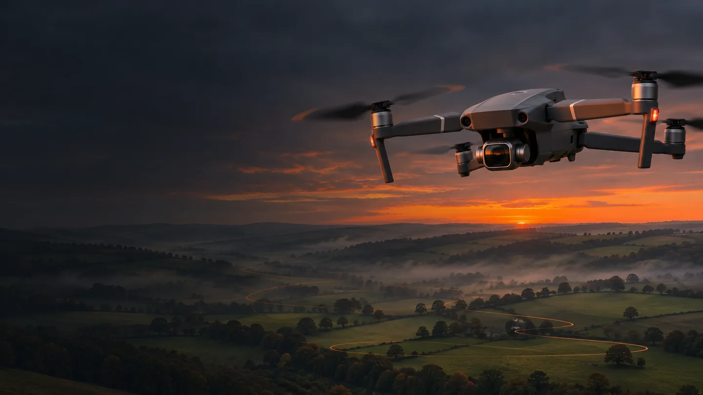
The Mavic 2 Pro can record visible patterns: lodging, uneven emergence, colour differences, bare patches, standing water and access damage. Similar-looking patches can have different causes. Light, soil background, growth stage and exposure can all change the appearance. Record weather, recent operations and crop conditions alongside the flight so later comparisons have context.
The geometry behind a useful photograph.
Ground sampling distance (GSD) is the approximate ground length represented by one image pixel. Fly lower and each pixel covers less ground, but the camera sees a smaller footprint: more lines, more photographs, more time. Fly higher and coverage improves while fine detail decreases. Neither option fixes a blurred image or poor overlap.
The calculator uses nominal Mavic 2 Pro still geometry: a 13.2 × 8.8 mm sensor, 10.26 mm physical focal length and 5472 × 3648 image. The 28 mm specification is a full-frame-equivalent angle-of-view description, not the focal length to insert into these equations. The 8.8 mm number is the sensor height; using it as this camera’s focal length would overestimate coverage.
GSD in cm/pixel = footprint width ÷ 5472 × 100
Forward trigger spacing = footprint length × (1 − forward overlap)
Flight-line spacing = footprint width × (1 − side overlap)
Assume a level surface, a nadir camera (−90°), full-resolution uncropped stills and the image’s long edge across the flight line. This is an idealised geometric model. Real lens calibration, terrain and aircraft attitude introduce differences; camera-derived GSD is not an accuracy certificate.
| Height above surface | GSD | Footprint W × L | Photo spacing | Line spacing |
|---|---|---|---|---|
| 60 m | 1.41 cm/px | 77.19 × 51.46 m | 10.29 m | 19.30 m |
| 80 m | 1.88 cm/px | 102.92 × 68.62 m | 13.72 m | 25.73 m |
| 100 m | 2.35 cm/px | 128.65 × 85.77 m | 17.15 m | 32.16 m |
80/75 is a starting point, not a magic spell
Forward overlap links photographs along a line; side overlap connects neighbouring lines. Together they give matching features multiple viewpoints. Crops are difficult because leaves move and repeated rows can look alike. Increase overlap when the subject needs it, but recognise that more nearly identical images cannot compensate for movement, missing viewpoints or featureless surfaces.
Plan extra coverage around the area you intend to deliver, while respecting permission and flight boundaries. The outermost photographs often have weaker reconstruction support. A taller crop or rising ground reduces the effective height above the photographed surface and shrinks the footprint; a route at constant take-off-relative altitude does not guarantee constant GSD or overlap.
Build a grid the camera can keep up with.
- Define the deliverable and legal operating area. Draw the field boundary in Hub’s area-mapping tool, after selecting the correct aircraft/app path. Keep the working grid inside a permitted, visible area. Large fields may need several separately supervised flights and launch positions.
- Choose height above the photographed surface. Begin with a modest test area at 60–80 m where lawful and appropriate. Inspect terrain changes and the actual altitude reference. A flat-field example is not a terrain-following instruction.
- Set the grid direction. Align long runs with the field where practical to reduce turns. Consider the wind and the return leg, not just outward speed. Keep turn space clear and ensure the camera footprint covers the required area.
- Set 80% forward and 75% side overlap as the initial plan. For crops, complex surfaces or uncertain conditions, a denser grid may be justified. Inspect the generated flight lines and their edge coverage before saving.
- Choose still format and a feasible capture interval. JPEG is a practical first mapping format. Keep the same settings throughout. Do not record video during the still mission. Original Litchi’s photo-interval behaviour and resets at waypoints mean you must check the actual spacing across turns.
- Open the saved route in original iOS Litchi. Verify the generated waypoints, heights, line direction, gimbal, interval and speed. Hub’s newer camera models and app-specific exports do not guarantee an equivalent aircraft configuration. If capture settings have not transferred, configure supported capture in the app and test it before the main grid.
- Fly a small verification strip. Count the actual photographs and inspect timestamps and sharpness. Confirm that the interval holds while the aircraft is moving and the card buffer is busy. Then fly the full approved plan with a tested reserve and continuous supervision.
| Capture choice | Distance between images | Forward overlap | Practical result |
|---|---|---|---|
| Ideal target: 2.74 seconds | 13.72 m | 80% | A calculated maximum interval, not an arbitrary DJI setting. |
| JPEG every 2 seconds | 10 m | 85.4% | Meets the 80% target if the camera sustains the cadence. |
| JPEG every 3 seconds | 15 m | 78.1% | Falls short of the requested 80%. |
| RAW every 5 seconds | 25 m | 63.6% | Too widely spaced at this speed. |
| RAW 5 seconds at ≤2.74 m/s | ≤13.72 m | ≥80% | Slow down and verify the actual recording interval. |
Sharpness earns its keep
Use a short exposure appropriate to speed, light and image scale. At 5 m/s and 1/1000 s, ideal forward motion during exposure is 5 mm—about a quarter pixel at 80 m. That is a useful planning check, not a universal shutter prescription. Keep ISO sensible, focus consistently and inspect sample photographs at 100% before committing to a large capture.
Remove cinematic ND filters if they prevent the faster exposure you need. Use stable white balance and avoid drastic exposure jumps between rows. Prefer steady light and limited wind; rapidly moving cloud shadows can create seams, and wind-driven crops may not reconstruct cleanly. The electronic rolling shutter is a separate distortion mechanism: a faster shutter reduces blur but does not turn the camera into a mechanical/global-shutter model.
How hundreds of images become one map.
- Find shared detailSoftware detects repeatable features and matches them between overlapping photographs.
- Solve the camerasBundle adjustment estimates camera positions, orientations, lens parameters and scene geometry together.
- Build the surfaceAdditional image evidence reconstructs dense detail and the surface needed for orthorectification.
- Place every pixelPhotographs are projected onto that surface, blended and exported into a georeferenced orthomosaic.
An orthomosaic is more than a panorama laid flat. Relief and camera perspective are accounted for using the reconstructed geometry, so locations can be placed consistently in a coordinate system. The quality of that geometry matters: repeated crop textures, moving leaves, reflective water and missed strips can create holes or warped areas even when the overview looks attractive.
Your Apple Silicon Mac workflow
Current WebODM supports Apple Silicon and offers free official installers. It now uses ODX and is independent of OpenDroneMap; older tutorials can describe a different installation or engine. Start from the official WebODM download page. The current Mac installer manages a Docker-based setup—follow its current macOS and Docker instructions rather than substituting old Intel commands.
- Create a project folder with
01_originals,02_working,03_outputsand04_quality. Copy the original card files and preserve EXIF. Keep an independent backup before deleting anything from the card. - Inspect every image quickly, then examine representative frames at full resolution. Separate take-off photographs, sky frames and obvious failures. Do not delete so many “similar” pictures that you destroy the overlap the software needs.
- Launch WebODM, create a project and add one coherent dataset. For your 16 GB Mac, begin with roughly 50–100 good images and a sensible/default quality preset. Keep ample free disk space, close memory-heavy apps and leave RAM for macOS. Larger projects may need more memory or remote processing.
- Add surveyed control and independent checkpoints if you have them. Confirm coordinate systems and height references. A wrong CRS or vertical datum can create a beautifully consistent error across the whole project.
- Process, then inspect the reconstruction and report. Look for disconnected areas, unaligned cameras, gaps, double edges and stripes. Re-fly a missed area when needed; do not disguise the gap with a painted patch.
- Export the georeferenced orthophoto GeoTIFF, quality report and any needed point cloud or elevation output. Keep processing options with the project, so a later visit can be compared fairly.
Turn the output into something useful.
Open QGIS and drag in the GeoTIFF, or choose Layer → Add Layer → Add Raster Layer. A correctly georeferenced orthophoto already contains positioning information; it does not need manual placement with the Georeferencer. Check that the location is plausible before measuring anything.
Set a suitable project coordinate reference system and explicitly review measurement units and ellipsoid settings. QGIS commonly measures on an ellipsoid; selecting a projected CRS does not by itself make every measurement planar. Record the method used, especially if comparing areas from different systems.
- Create a polygon layer for the area of interest and a point layer for observations to check on foot.
- Digitise visible features at a sensible scale. Distinguish an operational field outline from a legal property boundary: the photograph cannot establish title.
- Label possible wet patches, crop gaps or access issues as observations, not confirmed diagnoses. Include the flight date and the limits of the source.
- For repeat visits, align datasets using stable control and compare like-for-like conditions. Different sun angles or crops can imitate change.
- Export a readable map with scale, orientation, CRS, source date and quality notes. Deliver the interpretation alongside the image, so the next person understands what it can and cannot support.
A crisp map can still be in the wrong place.
Resolution describes detail; accuracy describes agreement with reality. At 80 m the nominal pixel size is about 1.88 cm, but consumer GNSS camera positions may leave metre-scale absolute errors. A sharp fence line can therefore be very clearly misplaced. Relative shape, absolute position and elevation accuracy are separate questions.
Ground control points help constrain the reconstruction. Checkpoints are independent surveyed locations withheld from that fit, used to test the result. Spread control around the perimeter, through the centre and across changes in elevation. Use visible targets and a survey method appropriate to the accuracy being claimed. Measuring the targets with an ordinary phone does not create survey-grade control.
Review horizontal and vertical checkpoint residuals, outliers and spatial patterns. Report the actual achieved result and the checking method. A low residual on points used to fit the model is not the same as independent validation. Current WebODM supports checkpoint labelling with a CHK- prefix; follow its input-format instructions precisely.
Drainage deserves particular care
A DSM follows visible surfaces, including crops, roofs and trees. A generated DTM attempts to identify ground and interpolate it, but cannot see soil hidden beneath dense vegetation. A very small vertical error can reverse an apparent shallow drainage gradient. Use aerial observations to identify where a proper ground investigation is needed; engineering design, legal boundaries and defensible volumes require suitable control and professional judgement.
Go to the source.
Primary documentation, specifications and research checked on 19 November 2026. Recheck before installing software or flying.
- DJI · Mavic 2 specifications
- Alfio et al. · Mavic 2 Pro camera geometry (Table 2)
- PIX4D · supported camera database
- Litchi Hub · current planner and release history
- Litchi · original app help and supported aircraft
- WebODM · flying and image acquisition
- WebODM · official installers and Apple Silicon support
- WebODM · installation and hardware guidance
- WebODM · ground control and checkpoints
- WebODM · digital elevation models
- QGIS · map view and measurement settings
- NASA · why NDVI needs near-infrared